|
|
| Line 73: |
Line 73: |
| '''MEASURING MICROBIAL GROWTH AS A<sub>590 nm</sub>''' | | '''MEASURING MICROBIAL GROWTH AS A<sub>590 nm</sub>''' |
| The intensity of color change is monitored in each of the wells by taking spectrophotometer readings once a day at A<sub>590 nm</sub>. You will come in daily to collect these data until a peak absorbance is reached on more than 2 consecutive readings, this will likely require daily readings for a week. You must not miss more than 1 consecutive day. Make sure that you take a photo of your plate against a white background on the final day of measurement.<BR><BR> | | The intensity of color change is monitored in each of the wells by taking spectrophotometer readings once a day at A<sub>590 nm</sub>. You will come in daily to collect these data until a peak absorbance is reached on more than 2 consecutive readings, this will likely require daily readings for a week. You must not miss more than 1 consecutive day. Make sure that you take a photo of your plate against a white background on the final day of measurement.<BR><BR> |
|
| |
|
| |
| [[Image:Plate-biologCarbon.jpg]]<BR><BR>
| |
|
| |
| '''Using the SpectraMax 340PC<sup>384</sup> Microplate Spectrophotometer and SoftMax Pro version 4.0™ software'''<BR>
| |
|
| |
| ===''' Spectramax 340PC :'''===
| |
|
| |
| '''Molecular Devices Spectramax 340PC instructions'''<BR><BR>
| |
| [[Image: Spectramax340PC2.jpg]]
| |
| [[Image: Switch.jpg]]<BR>
| |
| Turn on the Spectramax 340PC spectrophotometer using the switch located next to the plug in the back on the right hand side (as you face the spec). The drawer will open. The drawer may, or may not, close on its own. If it doesn't, close it by pressing, once, the DRAWER button found on the Spectramax control panel (pictured in purple on the instrument photo below). It is important to keep the drawer closed as much as possible to prevent dust from entering the spectrophotometer. The machine will automatically start a required calibration. Allow up to 10 minutes for the Spectamax340PC to warm up after the calibration and BEFORE you attempt to insert your plate.<BR><BR>
| |
| [[Image: Drawerbutton.jpg]]<BR>
| |
| The computer should be on. (If not, turn it on using the on/off switch on the processor on the floor).<BR><BR>
| |
| After the spectrophotometer finishes its start-up calibration, the drawer will open. If it doesn’t close on its own, close it by pushing ONCE the “drawer” button on the face of the spectrophotometer. <BR><BR>
| |
| When the warm up period is over, double click on the SOFTmaxPRO4.0 shortcut on the desktop of the computer. An “untitled” document will open on the computer screen called Default Tutorial 1.<BR><BR>
| |
| The draw may open again, or you can open it manually by pushing the DRAWER button ONCE. (Drawer button is found on the Spectramax control panel--as pictured in purple on the instrument photo above.)<BR><BR>
| |
| Position your 96 well plate into the tray drawer so that it fits securely in the holder and the well A1 is to the top left. Close it using the DRAWER button .<BR><BR>
| |
| [[Image: Screenshot1.jpg]]<BR>
| |
| Double Click the setup button located beside Experiment 1:
| |
| [[Image: Triangle.jpg]]<BR>
| |
| Plate #1 . set up
| |
| A new window will open called Instrument Settings. The icon ENDPOINT will be active.<BR><BR>
| |
| [[Image: WavelengthSET.jpg]]<BR>
| |
| Set the correct wavelength (590 nm for our Biolog®: carbon source plates). Click OK<BR><BR>
| |
| You will see a table representing a 96 well plate under EXPERIMENT #1. The spec is ready to read all the wells in a 96 well plate. <BR><BR>
| |
| In the upper toolbar menu at the top of the screen click READ. <BR><BR>
| |
| '''Troubleshooting:''' If the READ button is gray and won’t let you start the read, check for a red X over the PORT SERIES icon to the left of the READ button. It indicates NO PORT SELECTED. If so, click on this icon and select series port: COM 2 from the drop down menu. Click OK. (The drawer may open and you will need to close it).<BR><BR>
| |
| You will hear the spectrophotometer slit lamp passing over the plate to "read" it, meaning that it is measuring absorbance at the nm wavelength best for detecting purple colored pigments (590 nm). The purple color formation is a function of the total redox reactions that occurred in the well as the microbes use each carbon source metabolicaly and change the colorless form of the dye, 5-cyano-2,3,-ditolyl tetrazolium chloride (CTC), to a purple- colored product. <BR><BR>
| |
| The drawer will open when the readings are completed. Remove your plate and CLOSE the drawer using the DRAWER button on the face of the spectrophotometer. It is important to keep the drawer closed as much as possible to prevent dust from entering the internal parts of the machine. <BR><BR>
| |
| A new screen will appear with your recorded data in a 96 well template.<BR><BR>
| |
| [[Image:Spectramax1A.jpg]]<BR>
| |
|
| |
| As a safety precaution, immediately export these data on the computer desktop to the BISC folder for your lab section. Use File: Import/Export: Export . Be sure to label the file with your soil sample code and day of reading. <BR><BR>
| |
| Now save the data in EXCEL: HIGHLIGHT and COPY all the data in the 96 well template.<BR><BR>
| |
| Open a new Excel spreadsheet by clicking Start: Programs: Excel<BR>
| |
|
| |
| Paste the data from the 96 well template: EDIT: PASTE SPECIAL: TEXT into the Excel spreadsheet. This is a very important step because it aligns the cells properly.<BR><BR>
| |
| Label the wells in the spreadsheet A-H and 1-12.<BR><BR>
| |
| [[Image:Excel1a.jpg]]<BR>
| |
| Add identifying information to the worksheet title including: Biolog/590 nm: Date, Soil Sample ID code: Group color and Lab Day.<BR><BR>
| |
| Click Save As and rename the file with your group’s soil sample code and lab day.<BR><BR>
| |
| Close the Spectromax software. DON'T SAVE! (You have already saved and exported adequately.)<BR><BR>
| |
| Because the instrument computer is not networked, you will have to Save the excel spreadsheet to a FLASH DRIVE. If you don't have your own, there should be one in the USB port in the front of the computer processor (found on the floor under and to the left of the spectrophotometer). This one is provided for all BISC209 students. If the flash drive is missing, look to see if the last user left it connected to the Mac computer on the Instructor’s bench. If it is not there, you will have to send a message to the class through Forums in Sakai to see if someone took it home by mistake and email your instructor. <BR><BR>
| |
| If you have a flash drive available, open Excel and use the FILE drop down menu to SAVE AS: (provide an identifying title with your soil sample code letter and your team color and lab day) and SAVE TO REMOVABLE DISK (E), BISC 209-2011 folder: Lab section (TUES OR WED) folder. <BR><BR>
| |
| To remove a Flash Drive from a PC: Close the Excel document, you created, and click on the icon with a green arrow in the far right of the toolbar. A new screen will open “Unplug or eject hardware”. Click stop. In the “stop a hardware device” screen, highlight “generic volume device : E”. Click OK. The final screen tells you that it is safe to remove device. Click OK and Remove the Flash Drive from the computer.<BR><BR>
| |
| Now post your data in the google doc-linked through our lab SAKAI site. The file is called: BIOLOG-CMD_calc&GraphTEMPLATE_2012: To do this:<BR>
| |
| Take the Flash drive over to the Instructor’s Mac computer at the front of the lab and insert the flashdrive.<BR>
| |
| You will see an image appear on the desktop of the Mac.<BR>
| |
| Click to open it and find your data.<BR>
| |
| Save the daily data in to a folder for your soil sampling site on the desktop AND post it to a google spread sheet found in the Data folder in Resources in SAKAI<BR>
| |
| When you have saved, drag the FLASHDRIVE icon to the TRASH and wait for it to disappear from the desktop.<BR>
| |
| REMOVE THE FLASH-DRIVE from the Instructor computer AND RETURN IT TO THE USB PORT ON THE SPECTROMAX PROCESSOR WHERE YOU FOUND IT!!!<BR>
| |
| Turn off the SPECTROMAX instrument using the on/off switch on the back of the computer.<BR>
| |
| DO NOT turn off the computer but do close all the open windows. <BR>
| |
| PRECAUTION: If you haven’t saved your data and another group reads their plate, your data will be overwritten and lost.<BR><BR>
| |
|
| |
| '''DATA COLLECTION'''<BR>
| |
| We have provided you with a Google doc spreadsheet called '''BIOLOG-CMD_calc&GraphTEMPLATE_2012_Tues_siteA (or B, or C, and _Wed_siteD, or E, orF)''' You will find a link to this EXCEL spreadsheet template in SAKAI. Please copy and paste your daily data after each reading into this template. You will have to carefully copy and paste the day's absorbance readings to the template. Be sure to use the correct one for your team! It is crucially important that you align the right carbon source to its value (don't forget water) and get the right well numbers transferred to the appropriate position on the Worksheet DAY (1, 2,etc) in the template workbook. Note that the Template contains a separate worksheet (tabs on the bottom) for each day within the full workbook. Make sure that you fill out the appropriate day (DAY 0, 1, 2 etc). If you miss a day, leave that page blank.
| |
|
| |
| The Google Doc is pre-formatted with the calculations for these data. It includes the formulas to average replicate measurements each day and it will automatically subtract the background (readings in the water wells). There is a normalization for background that will be subtracted automatically (this threshold absorbance is 0.25 for each carbon source). We hope that including these pre-made calculations in the template will make your calculation of community metabolic diversity (CMD) and the data analysis of carbon source utilization patterns relatively uncomplicated. Please make sure you understand the EXCEL performed calculations. When you are sure that your data has been copied correctly into the appropriate template day, you will notice that the built in calculations will provide a final average absorbance reading for each substrate.
| |
|
| |
| Fill in the last column labled: '''SCORE 1 for wells with OD above 0.0'''. Once you fill in this final column, the template will calculate the total number of positive wells out of 31 for you and the SUM will appear in a cell below your data. This is the CMD for that day.
| |
|
| |
| Copy this number and use paste special to paste the value next to the appropriate day in the table on the last TAB of the workbook (CMDtable&graph).
| |
|
| |
| '''GRAPHING THE CMD DATA:'''<BR><BR>
| |
| The graph of our community metabolic diversity (CMD) is built into the last page of the Workbook template: You will observe this figure for the calculated soil sample's CMD values on the y axis versus time on the x. It provide a sense of the time frame for the community to begin using the carbon sources and by day 7 how many different sources out of 31 were used: The community functional metabolic richness in carbon source utilization. What is important about this graph in providing evidence for our hypothesis that a soil microbial community must be able to utilize a wide variety of carbon sources to support and maintain its abundance?<BR>
| |
|
| |
| '''What else can we learn from assessing Community Metabolic diversity (CMD)'''<br>
| |
| CMD is calculated by summing the number of positive responses (wells with a positive A<sub>595 nm</sub> value after all the corrections) at each incubation time. CMD is a simple way to represent the total number of substrates able to be effectively metabolized by the microbial community. It's a measure of diversity in use of carbon sources but '''it does not identify the carbon substrates or help us find a pattern of preferred substrates'''.<BR><BR>
| |
|
| |
|
| '''Carbon source utilization pattern:'''<BR> | | '''Carbon source utilization pattern:'''<BR> |
| Since CMD analysis does not provide specific information about the pattern of carbon substrates used in your soil community, how could you examine the pattern of use of carbon sources? You could plot on a column graph the average A<sub>590 nm</sub> absorbance of the three replicates (with error bars) on the final day of data collection on the y axis and the 31 different carbon sources on the x axis in one figure. (Remember that there is no such thing as a negative value for Absorbance so count anything that is less than zero as zero. Why might you seem to have a negative value?). Should you arrange those carbon sources in the order they are on the BIOLOG plate or is there a better way to organize them on your graph to show your main message(s)? What kind of information do you need in the figure legend? <BR><BR>
| | How do we analyze our data? You could plot on a bar graph the average A<sub>590 nm</sub> absorbance of the three replicates (with error bars) on the final day of data collection on the y axis and the 31 different carbon sources on the x axis in one figure. (Remember that there is no such thing as a negative value for Absorbance so count anything that is less than zero as zero. Why might you seem to have a negative value?). Should you arrange those carbon sources in the order they are on the BIOLOG plate or is there a better way to organize them on your graph to show your main message(s)? What kind of information do you need in the figure legend? <BR><BR> |
|
| |
|
| Can you think of other ways to illustrate functional metabolic diversity in your soil community?<BR><BR> | | Can you think of other ways to illustrate metabolic diversity of your isolates?<BR><BR> |
M465

Carbon Source Utilization Profiling:
Carbon Source Utilization
You have learned in other courses about the importance of carbon fixation by autotrophic photosynthetic plants. The inability to make carbon-carbon bonds and, therefore, to utilize carbon dioxide as a carbon source, is problematic for heterotrophic species including humans and all other animals. Fortunately there are bacteria that, like plants, are autotrophic and photosynthetic, although many others are heterotrophic, like us. Unlike us, however, bacteria are extremely diverse in the types of carbon sources they can use metabolically. Bacterial communities both compete and co-operate in utilization of available sources of essential, useable carbon. The health and longevity of the community is dependent on a continuous supply of useable carbon for all its members. Your investigation on carbon source profiling will identify carbon sources that can be utilized by your isolates under the conditions we provide them.
Carbon source patterns using BIOLOG™ Ecoplates
Observing patterns of substrate utilization across isolates can provide evidence of functional capabilities of that microbe in its community context. Additionally, understanding how metabolic substrates can be used in the communities can help us understand the stability or flexibility of that ecosystem. Carbon sources are crucial anabolic raw materials for heterotrophic microbial growth. Microbes vary enormously in their ability to make use of carbon in different forms.
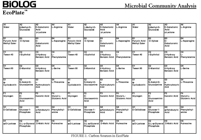
In the following assay, you will use your isolates, inoculated directly into the single carbon source wells of microtiter plates followed by spectrometric quantification of growth. If one or your microbes can use a particular carbon substrate, the metabolism of that carbon source is accompanied by a reduction of water-soluble colorless Tetrazolium salts (WTS) to become reduced purple formazans. WST-1 and in particular WST-8 (2-(2-methoxy-4-nitrophenyl)-3-(4-nitrophenyl)-5-(2,4-disulfophenyl)-2H-tetrazolium (MTT), are reduced outside of the cells. They combine with an electron mediator (phenazine methosulfate (PMS)), to yield a water-soluble purple product called formazan that can be measured spectrophotometrically at 590 nm. The color development is additive and directly proportional to the metabolism of each carbon source so the development of forazan can be followed over time. The intensity of purple color as a pattern in the wells is used to determine the metabolic footprint of your isolate. We will the patterns to determine the metabolic diversity of your isolates (CMD). For these measurements to be meaningful, it is important to control for number of microbes, incubation time, and other microenvironmental factors as well as the requirement for saturating substrate and indicator concentrations. There are 31 carbon sources available on a BIOLOG plate. This set of substrates is far from exhaustive. However, these substrates were chosen for variety and are similar to many nutrients found in natural environments.

Scheme showing the reduction of MTT to formazan. Image created by Jenpen 21 September 2006
Source http://en.wikipedia.org/wiki/File:Mttscheme.png . Public domain use per Wikipedia Commons.
Colorless (2-(2-methoxy-4-nitrophenyl)-3-(4-nitrophenyl)-5-(2,4-disulfophenyl)-2H-tetrazolium) is reduced to purple formazan
The BIOLOG-ECO™ 96 well plates we will use contain 3 replicates of 31 carbon sources and three water control wells. The method for carbon source profiling that we are using is simple and rapid, but its interpretation must be carefully evaluated, recognizing that the methodology is imperfect. The references below discuss the pitfalls of the ecoplates in the context of community level analyses:
References and Resources: Biolog Carbon Source
• Garland, J.L., Mills, A.L. (1991) Classification and characterization of heterotrophic microbial communities on the basis of patterns of community-level-sole-carbon-source-utilization. Appl Environ Microbiol 57, 2351–2359.
• Garland, J.L. (1997) Analysis and interpretation of community-level physiological profiles in microbialecology. FEMS Microbiol Ecol 24, 289–300.
• Preston-Mafham, J., Boddy, l., Randerson, P.F. (2002) Analysis of microbial community functional diversity using sole carbon source utilization profiles-a critique. FEMS Microbiology Ecology. 42, 1-14.
PROTOCOL:
Measuring the optical densities of your cultures
Your overnight broth cultures should have some turbidity (growth). We will use optical density at 600 nm as a measure of growth. You will then normalize each of your isolates to the lowest measurement.
1. Vortex your cultures briefly to resuspend the bacterial growth.
2. Label 5, 1.5 mL plastic eppendorf tubes with your isolate number. Label a final, 6th tube, with the word "blank".
3. Using sterile technique, remove 500 uL of broth from each culture into the appropriate 1.5 mL tube. To the "blank" tube add sterile media appropriate to your isolate.
4. To each tube, add 500 uL of distilled, deionized water. You are therefore making a 1:1 dilution. Vortex to mix.
5. Label 6 cuvettes with your name and isolate number or "blank". Take the 1 mL solutions and pipette them into the cuvettes.
6. Using the spectrophotometers provided, measure the optical density at 600 nm (your instructors will show you how).
7. Based on your calculations, determine the normalizations necessary to make sure each of your isolates is inoculated at the same density. Use the spreadsheet called OD600_calcs.xlsx provided in "resources" on Oncourse
Carbon source utilization patterns using BIOLOG™ Ecoplates
Materials:
- 10 mM phosphate buffer (sterile, pH 7)
- P200 and P1000 micropipets with sterile tips
- Multichannel pipet (set to deliver 100 µL) and sterile tips
- BIOLOG EcoPlate™
- sterile plastic multichannel reservoir
Notes:
- Wear gloves throughout the entire protocol
- Do not cross contaminate your samples or the solutions
- Keep your work area clean: freshly disinfect your bench top before beginning
- Do not use a vortex at any point in this protocol unless it is specified that you should do so.
Perform all of the below in your laminar flow hood
1. Make your dilutions as per the spreadsheet.
2. You will be using a multichannel micropipet to inoculate your plates with your dilutions. Pour 10 mL of your diluted culture into a sterile reservoir.
3. Be careful to preserve the BIOLOG Eco™ plate's and its cover's sterility (eg. don't place it face down on your bench). Remove the cover and transfer 200 µL of the dilution into each each well of the 96 well BIOLOG plate. Check visually the consistency of the amount of diluted extract in the micropipet tips after you have drawn up your aliquots to determine that you have no bubbles and that the quantity to be dispensed is the same. If the pipet tips appear unevenly filled or you have bubbles, do not dispense the inoculum into the wells! Start over. If you are unfamiliar with the use of multichannel pipets, ask your instructor to observe your technique.
4. Replace the cover of the plate and label one side of the cover. DO NOT LABEL ON the top or bottom to avoid interference in the light passage during spectrophotometric readings. Use a piece of your colored tape and include your initials, the date, and the isolate number.
5. Take a time 0 reading at A590 nm using the BioTek Synergy H1 384 plate reader (your instructors will show you how)
6. After each reading, place your covered plate in the atmospheric conditions for your isolate (anaerobic or aerobic), and at 37C.
MEASURING MICROBIAL GROWTH AS A590 nm
The intensity of color change is monitored in each of the wells by taking spectrophotometer readings once a day at A590 nm. You will come in daily to collect these data until a peak absorbance is reached on more than 2 consecutive readings, this will likely require daily readings for a week. You must not miss more than 1 consecutive day. Make sure that you take a photo of your plate against a white background on the final day of measurement.
Carbon source utilization pattern:
How do we analyze our data? You could plot on a bar graph the average A590 nm absorbance of the three replicates (with error bars) on the final day of data collection on the y axis and the 31 different carbon sources on the x axis in one figure. (Remember that there is no such thing as a negative value for Absorbance so count anything that is less than zero as zero. Why might you seem to have a negative value?). Should you arrange those carbon sources in the order they are on the BIOLOG plate or is there a better way to organize them on your graph to show your main message(s)? What kind of information do you need in the figure legend?
Can you think of other ways to illustrate metabolic diversity of your isolates?


