User:Floriane Briere/Notebook/CHEM-496/2011/09/14: Difference between revisions
| Line 36: | Line 36: | ||
==Results== | ==Results== | ||
'''* Curve of the concentration (nM) as a function of the Absorbance at 595nm''' | |||
[[Image:14sept - Abs(595=f(concentration).png]] | [[Image:14sept - Abs(595=f(concentration).png]] | ||
| Line 46: | Line 46: | ||
So, the pure MPB solution has a concentration of 31.2nM (0.0312*1000 = 31.2nM). | So, the pure MPB solution has a concentration of 31.2nM (0.0312*1000 = 31.2nM). | ||
* Curve of the Absorbance as a function of the Wavelength (nm) | '''* Curve of the Absorbance as a function of the Wavelength (nm)''' | ||
[[Image:14sept - Absorbance = f(wavelength) v2.png]] | [[Image:14sept - Absorbance = f(wavelength) v2.png]] | ||
| Line 52: | Line 52: | ||
This curve is made with the 1/1000 diluted MPB solution measures. | This curve is made with the 1/1000 diluted MPB solution measures. | ||
* Curve of the molar absorptivity (ε) as a function of the Wavelength (nm) | '''* Curve of the molar absorptivity (ε) as a function of the Wavelength (nm)''' | ||
According to Beer-Lambert law, Absorbance = molar absorptivity (L.mol^-1.cm^-1) * concentration (M) * length of the cuve (cm) | According to Beer-Lambert law, Absorbance = molar absorptivity (L.mol^-1.cm^-1) * concentration (M) * length of the cuve (cm) | ||
Revision as of 06:55, 20 September 2011
| File:BDLlogo notext ir.png Project name | <html><img src="/images/9/94/Report.png" border="0" /></html> Main project page <html><img src="/images/c/c3/Resultset_previous.png" border="0" /></html>Previous entry<html> </html>Next entry<html><img src="/images/5/5c/Resultset_next.png" border="0" /></html> |
|
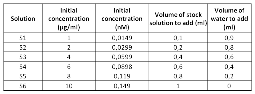
ObjectiveToday's experiment is to test the Bradford Assay technique which is going to allow us to determine the unknown proteins’ concentration of a solution. We are going to use 6 standards solutions of BSA whose concentrations are known. Then, thanks to a spectrophotometer, we’ll be able to determine the concentration of the MBP solution. Protocol
Results* Curve of the concentration (nM) as a function of the Absorbance at 595nm Red lines represent the Absorbance at 595nm of the 1/1000 diluted MPB solution. This curve allow us to determine the concentration of the 1/1000 diluted MPB solution. To draw this curve, we add to take into account that the Bradford Assay was made with 5/6 diluted solutions (because we added 1ml of solution to 200µl of Bradford reagent). According to this curve, the 1/1000 diluted MPB solution has a concentration of 0.0312nM (0.026*(6/5) = 0.0312nM). So, the pure MPB solution has a concentration of 31.2nM (0.0312*1000 = 31.2nM). * Curve of the Absorbance as a function of the Wavelength (nm) This curve is made with the 1/1000 diluted MPB solution measures. * Curve of the molar absorptivity (ε) as a function of the Wavelength (nm) According to Beer-Lambert law, Absorbance = molar absorptivity (L.mol^-1.cm^-1) * concentration (M) * length of the cuve (cm) NotesThis area is for any observations or conclusions that you would like to note.
| |


