Leanne Kuwahara-Week 11
Purpose
To simulate a chemostat using MATLAB and compare the results to a steady state outcome.
Background
- Chemostat: a reactor used for growing cell cultures
- Nutrients (media) added at a constant inflow rate
- Nutrients held at fixed concentrations
- Effluent removed at a rate equivalent to the inflow rate
- Effluent concentration DEPENDS on time
- Volume in chemostat held constant
- Assumed that contents of chemostat are well mixed (uniform concentration throught reactor)
- Thus, all cells have EQUAL access to nutrients
- Parameters:
- Q: volumetric inflow rate (vol/time)
- V: volume in chemostat (vol units)
- q = Q/V: dilution rate (1/time)
- u: feed concentration (concentration units)
- y(t): concentration of nutrients
- Rate of change of nutrients = inflow rate - outflow rate - rate consumed in tank
- Modeling Conservation of Nutrient Mass (dy/dt):
- qu: inflow rate (assumed to be CONSTANT over time)
- qy(t): outflow rate
- Er(y/K + y)x(t): consumption rate/rate of metabolism
- Michaelis-Menten model
- x: concentration of yeast cells
- E: unit conversion rate between biomass and nutrient concentration
- r: Maximum rate of system (Max specific growth rate)
- K: Nutrient concentration at which the reaction rate is half of Vmax (r)
- Modeling Cell Population (dx/dt):
- Net growth rate is dependent on nutrient level [y(t)]
- Consumption model depends on size of population
- Net growth rate is dependent on nutrient level [y(t)]
- In EQUILIBRIUM, models are set equal to ZERO
- x CANNOT be 0 (as this would mean the cell population was extinct)
- Nutrient concentration at equilibrium: y = qK/(r-q)
- Cell concentration at equilibrium: x = (u-y)/E
- The steady-state nutrient concentration is INDEPENDENT of the feed rate (u), while the cell population DEPENDS LINEARLY on u
- x CANNOT be 0 (as this would mean the cell population was extinct)
Protocol
- Solving for steady-state cell biomass (x) and nutrient mass (y):
- Parameters used:
- q = 0.10 (1/hr)
- u = 5 (g/L)
- E = 1.5
- r = 0.8 (1/hr)
- K = 8 (g)
- Parameters were plugged into y = qK/(r-q) and x = (u-y)/E to solve for cell biomass and nutrient mass (g) at equilibrium
- Parameters used:
- The mass calculated in number 1 were divided by 2 (L) to obtain the steady-state concentration (g/L) of cells and nutrients
- MATLAB files chemostat_script.m and chemostat_dynamics.m were used to simulate the system dynamics
- Same parameters were used in simulation
- Results from simulation were compared to the calculated values
- Same parameters were used in simulation
- Adding a Second Y-axis
- yyaxis left/right did not work
- Do no think this function is compatible with the 2014 version of MATLAB as it was released in 2016
- plotyy function did not work
- Over-layed a second y and x-axis
- plot2axes function did not work
- gave an error
- yyaxis left/right did not work
Results
- Calculated cell and nutrient mass:
- Cell biomass = 2.6g
- Nutrient mass = 1.1g
- Concentration in a 2L chemostat:
- [cells] = 1.5g/L
- [nutrients] = 0.5g/L
- MATLAB simulation
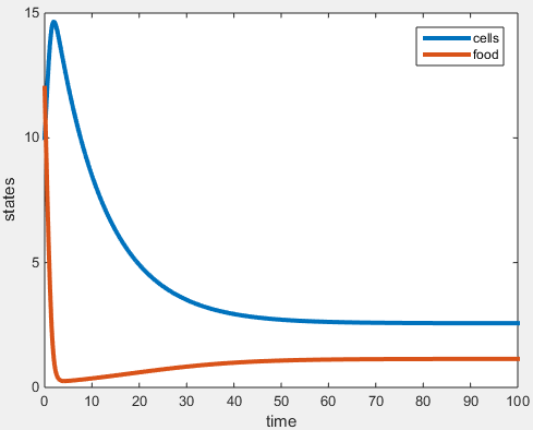
Figure 1. Plot generated in MATLAB simulation of a chemostat experiment.
- Plot demonstrates the chemostat goes to equilibrium around 50hr
- Plot shows equilibrium masses consistent with the calculated values (cells ~ 3g, nutrients ~ 1g)
Questions(Points of Confusion:
- I do not understand what in the code is assigned to the y-axis and what is assigned to the x-axis
- what are the units?? hours and g/L???
Data and Files
Conclusion
This aim of this experiment was to simulate a chemostat using MATLAB. The program produced a plot that successfully went to equilibrium, as expected with a chemostat experiment. Initially the cell population dramatically increased as the nutrient supply decreased. Once the nutrient concentration was near zero, the cell population peaked, and then decreased to a stead state around 3g. As the cell population decreased, nutrient concentration began to increase and also reached a steady state around 1g. These results demonstrate that MATLAB can be used to simulate chemostat experiments.
Acknowledgements
- Assigned Homework Partner: Fatimah Alghanem
- Except for what is noted above, this individual journal entry was completed by me and not copied from another source.
References
- Dahlquist, K. & Fitpatrick, B. (2019). "BIOL388/S19: Week 11" Biomathematical Modeling, Loyola Marymount University. Accessed from:Week 11 Assignment Page
Links
- Assignment Pages:
- Individual Assignment Link:
- Week 1- Create User Page: Leanne K. Kuwahara
- Leanne Kuwahara-Week 2
- Leanne Kuwahara-Week 3
- Leanne Kuwahara-Week 4/5
- Leanne Kuwahara-Week 6
- Leanne Kuwahara-Week 7
- No week 8 assignment
- Leanne Kuwahara-Week 9
- Leanne Kuwahara-Week 10
- Leanne Kuwahara-Week 11
- Leanne Kuwahara-Week 12
- No week 13 assignment
- Leanne Kuwahara-Week 14/15
- Class Journal Page:
- Class Journal-Week 1
- Class Journal-Week 2
- Class Journal-Week 3
- Week 4 shared journal assignment extended to week 5
- Class Journal-Week 5
- Class Journal-Week 6
- Class Journal-Week 7
- No week 8 assignment
- Class Journal-Week 9
- Class Journal-Week 10
- Class Journal-Week 11
- Class Journal-Week 12
- No week 13 assignment
- Class Journal-Week 14/15
- BIOL388 Home Page: BIOL388
- User page: Leanne K. Kuwahara
