Nathan R Beshai Week 2
From OpenWetWare
Jump to navigationJump to search
Nathan R. Beshai User Page
Nathan R. Beshai Template Page
Course assignments
Individual journal assignments
- Nathan R Beshai Week 2
- Nathan R Beshai Week 3
- Nathan R Beshai Week 4
- Nathan R Beshai Week 5
- Nathan R Beshai Week 6
- Nathan R Beshai Week 7
- Nathan R Beshai Week 8
- Nathan R Beshai Week 9
- Nathan R Beshai Week 10
- Nathan R Beshai Week 11
- The D614G Research Group Week 12
- The D614G Research Group Week 14
Class Journals
- Class Journal 1
- Class Journal 2
- Class Journal 3
- Class Journal 4
- Class Journal 5
- Class Journal 6
- Class Journal 7
- Class Journal 8
- Class Journal 9
- Class Journal 10
- Class Journal 11
- Class Journal 12
- Class Journal 14
Link to Brightspace and LMU's Homepage
Purpose of the Week 2 Assignment
- Observe how modeling can affect and influence the treatment of current and future pandemics and epidemics using COVID-19 as an example.
Methods and Results
Methods
- Visited the The role of applied math in real-time pandemic response: How basic disease models work YouTube video and noted any questions and observations that I had.
- After the questions were listed, this website titled The SIR Model was visited and the following questions were answered.
- What happens if initial I = 0?
- What does it mean that the red line increases so rapidly?
- What does it mean that the green line also rises rapidly, but not as rapidly?
- What does it mean that the green line reaches nearly 1,000?
- Visited disease modeling website Epidemix and chose the model type "Stochastic Homogeneous Mixing-ASF" because it infected pigs and had a greater culling rate.
- Took a screenshot of the initial graph without changing any parameters.
- Chose a couple of parameters to change. After each parameter change, the difference between the changed graph and the original graph was noted and its relation to the changed parameter was noted.
- Edited the "Define infection and transmission features" section and changed the number of infected units at the start of the stimulation from 1 to 10 and took a screenshot of the graph.
- Reverted parameters and edited the "Choose control strategy" section and chose a vaccination control strategy with a 0.5 proportion of vaccination units.
- Reverted parameters and edited the detection to culling (days) from 15 days to 5 days.
- Reverted parameters and edited infection to suspicion (days) from 30 days to 20 days.
- Reverted parameters and changed the "suspicion to detection (days)" from 5 days to 15 days.
- Reverted parameters and edited the "Define infection and transmission features" section and changed the daily number of effective contacts per unit from .62 to .40.
- Reverted parameters and edited the "Define host population features" section, changing the population to an open population with a duration of the presence of a unit in the population (days) to 25 days.
- Reverted parameters and edited the "Choose control strategy" section and chose a culling control strategy and reduced length of the symptomatic infectious period due to culling for 2 days.
- Reverted parameters and edited the "Define infection and transmission features" section and changed the mode of transportation from a frequency-dependent transmission to a density-dependent transmission.
- Reverted parameters and edited the "Define infection and transmission features" section and changed the number of latent days from 4 days to 10 days.
- Visited the article "Modelling the COVID-19 epidemic and implementation of population-wide interventions in Italy" and answered the following questions based on figure 1.
- How did the authors modify the simple SIR model to take into account features of the COVID-19 pandemic?
- What public health policy implications does their model have?
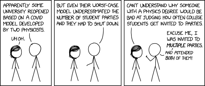
- Viewed the comic University COVID Model and commented on why it was so funny.
- Wrote a detailed scientific conclusion and summary detailing the importance of modeling applied to infections and specifically SARS-COV-2.
Results
- Questions in response to the The role of applied math in real-time pandemic response: How basic disease models work YouTube video.
- Why do we see different peaks when more babies are born, wouldn't the rates be constant since babies' birth rates are relatively constant?
- Shouldn't we re-open the country when the curve is far below the healthcare capacity and close when the rate reaches close to the capacity?
- Questions from The SIR Model.
- What happens if initial I = 0?
- If initial I (infected) = 0 then the number of people recovered and the number of deaths also equals zero. This is because a person who is not infected with a virus cannot recover from it or die from it. The number of people susceptible remains the same because although the virus hasn't infected anybody yet people can still be susceptible to it.
- What does it mean that the red line increases so rapidly?
- The red line indicates infected people so the reason it increases so rapidly is that the infection is highly contagious. This can be seen because the number of susceptible people quickly become infected people.
- What does it mean that the green line also rises rapidly, but not as rapidly?
- The green line represents people who were infected and recovered from the infection. The green line rises but not as rapidly because it has a quick recovery from the illness but it takes a shorter time to become infected with the infection than to recover from the infection.
- What does it mean that the green line reaches nearly 1,000?
- The green line reaching nearly 1,000 means that almost all the people who were susceptible and were infected recovered. The reason it did not reach 1,000 is that the infection either did not infect someone who was susceptible or that the person who became infected died from the infection.
- What happens if initial I = 0?
- Figures from Epidemix, the model type chosen was the "Stochastic Homogenos Mixing-ASF" model because it was sampling a pig population and displayed forced culling in infected animals.
- Figure 1: Initial Plot from the Stochastic Homogeonous Mixing-ASF Model.

- Without any changed parameters to the current model. The population of pigs presented with 99 susceptible pigs/infected, by the end of the 40 day period around 58 of the pigs died, around 22 of the pigs were infectious-symptomatic, around 15 were infected(latent), around 5 were infectious-asymptomatic, and 0 were still susceptible. This indicates that the disease is highly transmittable because all 100 that were susceptible became infected. It also shows that there is a high mortality rate with the infection because before the pigs were culled there was a 58 percent death rate with the infected pigs which would have increased without culling the pigs.
- Figure 2: Plot from the Stochastic Homogeonous Mixing-ASF Model with the changed the number of infected units at 10 instead of one.

- The change in a number of infected units to ten increased peak and caused more pigs to die before the 40 days mark. At the 40 day mark, around 96 of the 100 pigs were dead and only around 4 of the 100 pigs were still alive but infectious-symptomatic. This proves that the mortality rate is very high and if the simulation continued might be 100 percent. There were no Infectious-asymptomatic or infected(latent) pigs by the 40-day mark.
- Figure 3: Plot from the Stochastic Homogeonous Mixing-ASF Model with .5 Vaccinated Units in the Population.

- The .5 vaccination in the population reduced the number of susceptible to 50 pigs. Surprisingly, the mortality rate was not as high as in the figure without the vaccine. By the end of the 40 day period around 18 of the pigs died, around 8 of the pigs were infectious-symptomatic, around 5 were infected(latent, around 1 was infectious-asymptomatic, and 18 were still susceptible. This meant that with only half the population susceptible it takes a longer time for the pigs to get infected because the number of contacts with sick pigs is limited.
- Figure 4: Plot from the Stochastic Homogeonous Mixing-ASF Model with the gap between detection and culling increased from 5 days to 15 days.

- The extending of the days between detection and culling from 5 to 15 days increased the number of pigs who died from infection and decreased the number of infectious-symptomatic pigs to around 8 and decreased the number of infected (latent) pigs and infected-asymptomatic pigs to zero. Extending the days between detection and culling helped view that around the 43-day mark there were no more infected (latent) pigs and infected-asymptomatic pigs. When the separation was 5 days instead of 15, the number of days could not be viewed because it occurred around 43 days.
- Figure 5: Plot from the Stochastic Homogeonous Mixing-ASF Model reducing the infection to suspicion (days) from 30 days to 20 days.

- Reducing the number of days from the infection to suspicion reduced the knowledge about the infection. This shifted everything to ten days earlier. This also meant the data points decreased which gave us a smaller picture of the mortality rate and the other variables.
- Figure 6: Plot from the Stochastic Homogeonous Mixing-ASF Model increasing the gap of "suspicion to detection (days)" from 5 days to 15 days.

- Increasing the days between suspicion and detection broadened our view by increasing the data points of the model. This parameter did not change the data points but increased them. This helped get a better view of where the mortality rate was going and showed the decreasing number of Infectious-Symptomatic and increasing the number of dead pigs.
- Figure 7: Plot from the Stochastic Homogeonous Mixing-ASF Model with the effective contacts between the contacts reduced from 0.62 to 0.40.

- Reducing the number of contacts flattened the curve of susceptible pigs becoming infected. This can be seen because by the forty-day mark the number of susceptible pigs was still at around 30 with infected pigs or dead pigs at around 70 total. This is far lower than the initial graph with an effective contact rate of .62, as the number of susceptible pigs being around 1 or 2 and the infected pigs or dead pigs at around 99 or 98 pigs.
- Figure 8: Plot from the Stochastic Homogeonous Mixing-ASF Model changing the population to an open population with a duration of the presence of a unit in the population (days) to 25 days.

- Changing the parameter to an open system created a chance for susceptible pigs to be able to leave the population without being infected. This is why the number of susceptible pigs did not reach 0 but remained around 18 pigs by the end of the 40-day mark. This also decreased the number of dead and infected pigs because the number of susceptible pigs did not reach 0 pigs meaning that they were not infected. Something that this model doesn't show is the other systems that the pigs traveled to when they left because infected pigs also left which would infect other systems.
- Figure 9: Plot from the Stochastic Homogeonous Mixing-ASF Model changing to a culling control strategy and reducing the length of the symptomatic infectious period due to culling for 2 days.

- This parameter not only culled pigs at the 40-day marks but culled them after viewing symptoms for 2 days. This reduced the opportunity for pigs to infect other pigs because the symptomatic infected pigs were killed after two days of being symptomatic. This allowed for more pigs to refrain from being infected and remain susceptible for a longer period of time. However, this did not eradicate the infection because the asymptomatic infected pigs were also contagious and were not culled.
- Figure 10: Plot from the Stochastic Homogeonous Mixing-ASF Model changing the mode of transportation from a frequency-dependent transmission to a density-dependent transmission.

- The change between frequency-dependent transmission and density-dependent transmission was not too radical. The Density-dependent transmission caused the infection to spread slightly quicker than the frequency-dependent transmission. This means that the pigs in a more populated area were not getting infected a lot quicker than those with a higher frequency transmission.
- Figure 10: Plot from the Stochastic Homogeonous Mixing-ASF Model changing the number of latent days from 4 days to 10 days.

- This parameter had the largest effect on the graph because it flattened the infection curve the most. The number of latent days increased to ten kept the number of infected pigs to slightly under 60 pigs which were at 0 for the 4 latent day graph at day forty. The number of dead pigs and infected pigs was slightly above 40, whereas, they were at 100 for the 4 latent day infection.
- Figure 1: Initial Plot from the Stochastic Homogeonous Mixing-ASF Model.
- Questions from the article "Modelling the COVID-19 epidemic and implementation of population-wide interventions in Italy".
- How did the authors modify the simple SIR model to take into account features of the COVID-19 pandemic?
- The author's modeled the COVID-19 SIR model to emphasize how infectious the virus was, how it can go undetected, and how the mortality of COVID-19 was low. They did this by showing that every stage had a path to healing and that two of their variables were for individuals who did not even know they had coronavirus. These implications do not always apply. In the infection among the pigs above, the infection had an extremely high mortality rate.
- What public health policy implications does their model have?
- The public implications their model has are that there is not testing to everybody who is infected and even symptomatic. This means that people who had COVID-19 might not have even been diagnosed. On the contrary, another implication is that people who have no symptoms can be tested, even when there is no clinical reason to test.
- How did the authors modify the simple SIR model to take into account features of the COVID-19 pandemic?
- Why is the University COVID Model so funny?
- This model is funny because modeling the Coronavirus on a university requires estimating the number of contacts individuals have with one another and to model risk exposure. This model demonstrates that physics majors got the model wrong because they did not estimate how frequent non-physics majors actually left the room. This caused an outbreak to occur because people were gathering.


Scientific Conclusion
- This journal showed the importance of modeling when dealing with a pandemic or an epidemic. SIR models are tools that scientists can use to predict the mortality rate and infection rate a society has with different infections. Estimating parameters and variables is crucial because an incorrect estimation can cause a result that may have a negative effect on society. When creating COVID-19 Models, it is important to consider public implications. Whether or not the public adheres to stay at home orders or a face-mask policy can affect the results of the created model. It is also imperative that scientists work with politicians to work on a model that actually works with the population in the given area.
Acknowledgments
- Copied APA syntax and OpenWetWare syntax from the BIOL368/F20 Week 1 Page.
- Copied instructional questions and website links from the BIOL368/F20 Week 2 Page.
- Copied image formatting syntax from MediaWiki images.
- Watched the video and asked questions from the The role of applied math in real-time pandemic response: How basic disease models work YouTube video.
- Read the article and asked questions from "The SIR Model".
- Copied the Stochastic Homogeoneous Mixing-ASF model and edited parameters from Epidemix.
- Looked at figure 1 and asked questions based on the article Modelling the COVID-19 epidemic and implementation of population-wide interventions in Italy.
- Answered what was funny from University COVID Model.
- Used the Purdue owl to learn how to cite sources using the APA style.
- Lab partner this week was JT Correy and we collaborated choosing the Stochastic Homogeneous Mixing-ASF model to change the parameters.
- Referenced the Why Model article by Joshua Epstein for the Class Journal Week 2.
References
- OpenWetWare. (2020). BIOL368/F20:Week 1. Retrieved September 13, 2020, from https://openwetware.org/wiki/BIOL368/F20:Week_1
- OpenWetWare. (2020). BIOL368/F20:Week 2. Retrieved September 13, 2020, from https://openwetware.org/wiki/BIOL368/F20:Week_2
- MediaWiki. (2020). Help:Images. Retrieved September 14, 2020, from https://www.mediawiki.org/wiki/Help:Images.
- Fefferman, N. (2020, April 1). The role of applied math in real-time pandemic response: How basic disease models work. [Youtube Video]. NIMBioS. Retrieved from https://www.youtube.com/watch?v=Ewuo_2pzNNw&feature=youtu.be.
- XKCD. (2020).University COVID Model. Retrieved September 15, 2020, from https://imgs.xkcd.com/comics/university_covid_model.png.
- e-Mission: PANDEM-SIM. (2020). THE SIR MODEL. Retrieved September 13, 2020, from http://www.pandemsim.com/beta/SIRmodel.html.
- Epi-Interactive. (n.d). Epidemix Version 2. Retrieved September 14, 2020, from https://www.epidemix.app/#.
- Giordano, G., Et. Al. (2020). Modelling the COVID-19 epidemic and implementation of population-wide interventions in Italy. Nature Medicine, 30,855-860. https://doi.org/10.1038/s41591-020-0883-7.
- The Purdue Owl. (2018). Citation Chart. Retrieved September 15, 2020, https://owl.purdue.edu/owl/research_and_citation/using_research/documents/20180719CitationChart.pdf.
- Epstein, J. M. (2008). Why Model Journal of Artificial Societies and Social Simulation, 11 (12), Retrieved from http://jasss.soc.surrey.ac.uk/11/4/12.html.bak.
"Except for what is noted above, this individual journal entry was completed by me and not copied from another source"Nathan R. Beshai (talk) 11:35, 15 September 2020 (PDT)