User:Alexander T. J. Barron/Notebook/PHYC 307L Lab Notebook/e over m notes
e/m Ratio Lab
SJK 02:47, 23 October 2008 (EDT)

this is a very good notebook. You are missing, though, a mention of your data analysis code (matlab, presumably) and a link to the code.
Overall, I can tell that you spent a bunch of time acquiring these photos, then coming up with a way of analyzing them. It's an interesting method, not sure how much effort you had to put in versus just trying to make the measurements by eye? I'm impressed that you two set out to try out this new method. The photos are great!
Set up
Followed prescribed procedure, with added sophistication:
Power Supply for heater: SOAR DC POWER SUPPLY, model PS-3630
Connected voltmeter in parallel to measure the V for the heating coils PRECISELY at 6.200 V. This is a great improvement over the gross dial meter on the actual power supply.
Now we won't touch the knobs...
Rearranged, measured current from same supply: .727 A
Now for V on electrodes: 200.0 V
Current to coils: 1.199 A
OK, so Gold's manual is WRONG and the electrode voltage needs to be ~ 300 V like in the lab notes for this class...
NEW SET UP
Heater V and A same.
Electrode V = 299.9 V
Coil current = 1.196 A
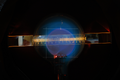
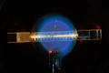
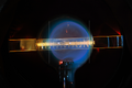
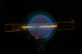
Lo and behold, a nice circle of green in the He.
- Alexander T. J. Barron 01:42, 16 October 2008 (EDT): Unfortunately, I noticed we didn't record the majority of our apparatus in terms of model numbers, exact configuration, etc. Something must have grabbed our attention.
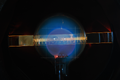
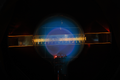
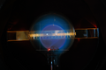
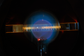
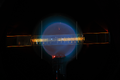
Data
| Constant V Trials | Corresponding Pictures |
|
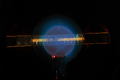
1) DSC_0006
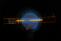
2) DSC_007
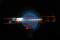
3) DSC_008
4) DSC_009
5) DSC_010
|
|


| Changing V and I Trials | Corresponding Pictures |
|
1) DSC_011
2) DSC_012
3) DSC_013
4) DSC_014
5) DSC_015
6) DSC_016
7) DSC_017
8) DSC_018
9) DSC_019
10) DSC_020
|
|


Qualitative Experiments
We performed this on the second period for this lab, with a different setup:
Same equipment, same config, with:
371.0 V to electrodes,
6.202 V to heater,
1.176 A to coils.
This produces a nice big, round e- path to play with.
Upon turning the bulb, we observe the helical motion of the e- path, with z direction according the z component of the initial velocity of the e-s (z being perpendicular to the Helmoltz coil plane). Initially, it seemed that one of the turns would create a split in the beam creating helices in both directions of z. Upon further inspection, the path seemed to follow the initial velocity z component and then bounce off the bulb to travel in the opposite direction.
We noticed that the radius of the electron path changed with change in the heater voltage. The B field and charge of electron don't change, so the the only thing that can cause a change in the Lorentz force is the initial velocity of ejected electrons. We didn't change the accelerating voltage, so the only seeming way the heater voltage could change the path radius would be significantly added velocity through ejection from the filament. The filament was glowing orange, and by Wein's Displacement Law,
[math]\displaystyle{ \lambda_{max} = \frac{b}{T}, }[/math]
with [math]\displaystyle{ b }[/math] = 2.897 768 5(51) x 10E–3 m K.
In this case, [math]\displaystyle{ \lambda_{max} }[/math] is around 590 nm. Wein's D. Law gives us [math]\displaystyle{ T }[/math] ≈ 4900 K.
I was going to compare the work function of Tungsten to the amount of energy given to the electrons through blackbody analysis, but I am not actually sure how to relate temperature of the filament to the energy of ejected electrons. I would hazard a guess that any extra kick given to the electrons would be insignificant in comparison to the accelerating potential of the gun.
I also thought heating up of He around filament might affect the speed of the electrons, but Dr. Koch didn't believe that would have much effect.
After reversing the supply poles on the Helmoltz terminals, we observe an opposite force on the e-s as opposed to the original setup. This is straightforward and expected- the B vector flipped direction, so the cross product (qv x B) flipped direction.
On to the Deflection Plates. Zero current in coils, as prescribed. Electrodes back to original polarity. When the plates are turned on, the beam curves up almost vertically. Upon inspection of the plate set up, the top plate must be positively charged because the Coulomb force FC = qE. q is negative in this case, so the e-s will approach the positively charged plate. Therefore, the top plate must be positively charged. We fooled with the accelerating potential, which powers the plates, and the degree of deflection doesn't seem to be altered much. The beam length does change appreciably, however, which makes sense from the accelerating potential's perspective. Since the plates are connected in parallel, change in voltage should change the degree of deflection of the beam. My explanation for not observing this phenomenon is that the change in E field between the plates is small compared to the change in v initial due to the same change in accelerating potential.
In order to test J. J. Thompson's mettle, we reversed the polarity on the plate jacks so the Lorentz force would counteract the plates' effect. It did, but not to a great degree. Larger parallel plates would have to be used, or a much higher potential, in order to full counteract the curving from the magnetic field.
Data Analysis
SJK 02:39, 23 October 2008 (EDT)
I think your method is pretty cool. And if there was a quick way of doing it, it may save a lot of students a bunch of eye strain. However, since I can't see the process, it's tough to know. I also am skeptical of your 0.01 pixel uncertainty. I think this is maybe what you were discussing below, but I can't quite understand. I think just looking by eye, the uncertainty should be several pixels. Plus, the whopper systematic error from the fact that it's not a circle anyway, and thus the measurement is probably biased.
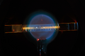
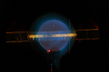
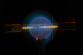
I used Adobe Photoshop's hue and saturation editors to make clarify the boundaries of the electron path, then the ellipse tool to overlay a circle approximating the outer edge of the path. I used guides snapped to the circle's edge, enabling me to draw a perfect square about each circle. Finding the diameter is then a cinch, using the ruler tool. I set all units to pixels, then measured 10 cm (from the center of one "5 cm" gradation to the other) according the the background ruler on the apparatus. I felt that was the largest width I could use without incurring too much optical distortion from the bulb, which one can see in the pictures near the bulb edge. With that conversion factor, I can find the radius in cm for each trial. This is why having a fine arts major roommate is a good thing!
The pictures I provide below are scaled down to decrease browser loading time. I took the pixel widths off much higher resolution pictures. Photoshop measures to hundredths of pixels, so my measurement error will be ± .01 px, for both the conversion value and the diameter value. I use both measurements in finding the radius, so their respective uncertainties both come into play. If I think about each uncertainty as a collection of small pieces of uncertainty (any one of which could be the true value of the measurement), their combination would would simply be the multiplication of both collections. Thus, my final uncertainty on Ri will be the two uncertainties multiplied.SJK 02:35, 23 October 2008 (EDT)
OK, so I don't understand what you're saying here...will have to talk about it in person
On second thought, that will decrease my overall uncertainty... but the idea sounded good. I believe the worst measurement would have the added maximum uncertainty of both measurements, so I'll use that.
I investigated the standard deviation route to finding error, but I don't believe that makes sense in this situation. If I had taken several measurements of Ri with Photoshop, then I could find random error on R for each iteration of i. Instead, I took one measurement roughly outlining the outer edge of the electron path for each iteration. Investigating the random error vs. the measurement uncertainty could be a good route to take for a final lab report. I'm not sure how one would include both random error and measurement uncertainty, though...
Ri Values
SJK 02:33, 23 October 2008 (EDT)
Looks like you needed a bigger range of currents?
| Constant V Trials | Measured Pictures | Measured Radius (Ri) |
|
1) ConstV01meas.tif:
|
|
R1 = 4.1796 ± 2.2684e-04 cm |
|
2) ConstV02meas.tif:
|
|
R2 = 4.2591 ± 2.2868e-04 cm |
|
3) ConstV03meas.tif:
|
|
R3 = 4.1848 ± 2.2868e-04 cm |
|
4) ConstV04meas.tif:
|
|
R4 = 4.1904 ± 2.2712e-04 cm |
|
5) ConstV05meas.tif:
|
|
R5 = 4.0871 ± 2.2868e-04 cm |
| Changing V and I Trials | Measured Pictures | Measured Radius (Ri) |
|
1) VIchange01meas.tif
|
|
R1 = 5.0195 ± 2.2868e-04 cm |
|
2) VIchange02meas.tif
|
|
R2 = 5.2482 ± 2.2868e-04 cm |
|
3) VIchange03meas.tif
|
|
R3 = 4.9509 ± 2.2868e-04 cm |
|
4) VIchange04meas.tif
|
|
R4 = 5.0022 ± 2.2867e-04 cm |
|
5) VIchange05meas.tif
|
|
R5 = 5.2192 ± 2.2841e-04 cm |
|
6) VIchange06meas.tif
|
|
R6 = 5.0765 ± 2.2867e-04 |
|
7) VIchange07meas.tif
|
|
R7 = 4.7340 ± 2.2842e-04 cm |
|
8) VIchange08meas.tif
|
|
R8 = 4.5400 ± 2.2843e-04 cm |
|
9) VIchange09meas.tif
|
|
R9 = 4.4654 ± 2.2841e-04 cm |
|
10) VIchange10meas.tif
|
|
R10 = 4.4531 ± 2.2895e-04 cm |
Charge-to-Mass Ratio
Pure Data Method
Dr. Gold's Lab Manual gives us
[math]\displaystyle{ B = (\frac{7.84}{10^4} \times \frac{weber}{ampere}) \times I, }[/math]
where [math]\displaystyle{ I }[/math] is the current through the Helmoltz coils.
The Lorentz Force is: [math]\displaystyle{ \vec{F_L} = q * [\vec{E} + (\vec{v} \times \vec{B})] = q\vec{v} \times \vec{B} }[/math] in this case.
Incidentally, the electron gun is inside the [math]\displaystyle{ \vec{B} }[/math] field, so [math]\displaystyle{ \vec{F_L} }[/math] is present in its full form inside the gun. The manual doesn't address this, and I don't know the actual construction of the gun, so I can't posit much effect. I would assume the gun is constructed to take into account the strengthening magnetic force as the electron accelerates to its final speed.
In theory, an electron moving through a [math]\displaystyle{ \vec{B} }[/math] field will travel in a circle due to [math]\displaystyle{ \vec{F_L} }[/math], since the acceleration [math]\displaystyle{ \vec{a} \perp \vec{v}. }[/math]
[math]\displaystyle{ \vec{F_L} }[/math] provides the centripetal force in this situation, so [math]\displaystyle{ \vec{a} = \frac{\vec{v}^2}{R}. }[/math]
Newton, or Isaac as I know him, declares [math]\displaystyle{ m\vec{a} = q\vec{v} \times \vec{B} = m\frac{\vec{v}^2}{R}. }[/math]
[math]\displaystyle{ \vec{v} \perp \vec{B} \longrightarrow \frac{q}{m} = \frac{v}{RB} }[/math]
[math]\displaystyle{ \frac{1}{2}mv^{2}=qV \longrightarrow v=\sqrt{\frac{2qV}{m}} }[/math]
[math]\displaystyle{ \frac{q}{m} = \frac{1}{RB}\sqrt{\frac{2qV}{m}} \longrightarrow quadratic formula \longrightarrow \frac{q}{m} = \frac{2V}{(RB)^2} = \frac{2V}{R^2(kI)^2}, }[/math]
where [math]\displaystyle{ V }[/math] is the accelerating voltage in the electron gun, [math]\displaystyle{ k = \frac{7.84}{10^4} \frac{weber}{ampere}, }[/math] and [math]\displaystyle{ R = R_i. }[/math]
Data Method Implementation
Error calculated as standard deviation of e/m ratio computed without taking error of V, I, or R measurements into account. Hopefully I'll be able to implement error propagation in future labs.
| e/m Ratio Constant Voltage | e/m Ratio Changing Voltage, Current |
|
[math]\displaystyle{ \frac{q}{m} }[/math] = 4.6573e11 ± 4.9646e10 [math]\displaystyle{ \frac{C}{kg} }[/math] |
[math]\displaystyle{ \frac{q}{m} }[/math] = 4.3653e11 ± 5.9377e10 [math]\displaystyle{ \frac{C}{kg} }[/math] |
Slope Method
I can also get the ratio by analyzing the slope of the graph of Ri vs. [math]\displaystyle{ \frac{1}{I} }[/math] for constant electron-gun voltage.
The method to find [math]\displaystyle{ \frac{q}{m} }[/math] is as follows:
[math]\displaystyle{ r^{2}(V)=(\frac{m}{e})\frac{2}{B^{2}}V }[/math]
[math]\displaystyle{ B=I \times k, k = \frac{7.84}{10^4} \times \frac{weber}{ampere} }[/math]
[math]\displaystyle{ r(\frac{1}{I})=\sqrt{\frac{2mV}{q}}\frac{1}{k}\frac{1}{I} }[/math] SJK 02:31, 23 October 2008 (EDT)
is there a typo here?
[math]\displaystyle{ slope = \sqrt{\frac{2mV}{q}}\frac{1}{k} }[/math]
[math]\displaystyle{ \frac{q}{m}=\frac{2V}{slope^{2}k^{2}} }[/math]
Thank you to Paul for laying out a lot of this slope-method LATeX.
Slope Method Implementation
SJK 02:29, 23 October 2008 (EDT)
I am not comfortable with any kind of fitting of this data. As you illustrate, it's not even convincing whether the slope is positive or negative! I don't know why that is, but to use this method, I'd want to take more data.
Also, what you want to do is force the linear fit to go through the origin, since your relation does not allow for an offset (infinite current should equal zero radius)
I didn't bother with my uncertainty, due to its insignificance compared to the difference in R values. With MATLAB's basic plot fitting GUI:
|
|
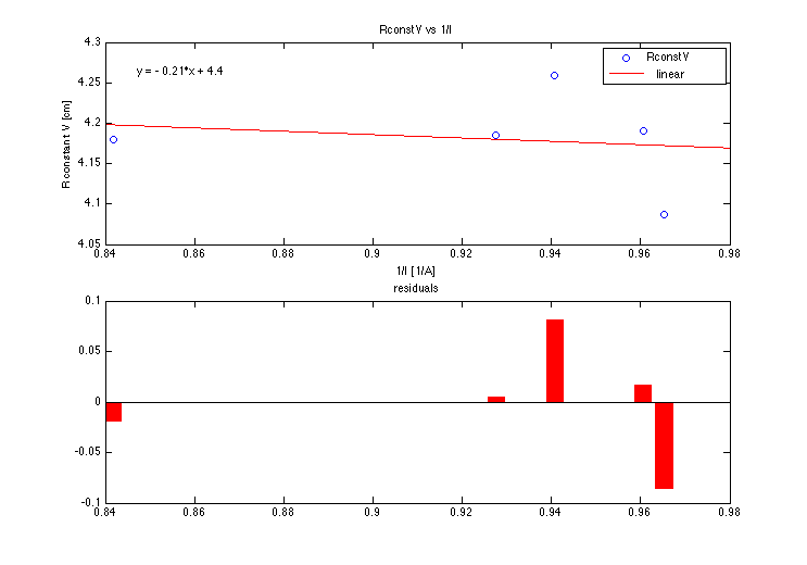
I first tried a least-squares linear fit with all of my data, but the rightmost data point seems to skew the fit more than is reasonable. See the residuals plot above. Because of this, I threw that "bad" point out (I can do that - it's my data hahaah) and fit again:
|
|
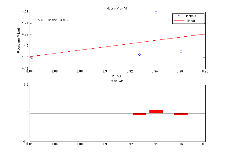
If one compares the residuals plots, I think the second fit is more reasonable.
| e/m Ratio Constant Voltage, Slope Method |
|
[math]\displaystyle{ \frac{q}{m} }[/math] = 1.2014e10 [math]\displaystyle{ \frac{C}{kg} }[/math] |
Comparison with Accepted Value
The accepted value of e/m is [math]\displaystyle{ -e/m_{e}= -1.758 820 150(44) \times 10^{11} {C / kg}. }[/math]
SJK 11:27, 20 October 2008 (EDT)
These values, compared w/ the accepted value, do not match your percent errors, and seem all over the place...lots of typos?
| e/m Ratio Constant Voltage | e/m Ratio Changing Voltage, Current | e/m Ratio Constant Voltage, Slope Method |
|
[math]\displaystyle{ \frac{q}{m} }[/math] = 4.6573e11 ± 4.9646e10 [math]\displaystyle{ \frac{C}{kg} }[/math] |
[math]\displaystyle{ \frac{q}{m} }[/math] = 4.3653e11 ± 5.9377e10 [math]\displaystyle{ \frac{C}{kg} }[/math] |
[math]\displaystyle{ \frac{q}{m} }[/math] = 1.2014e10 [math]\displaystyle{ \frac{C}{kg} }[/math] |
|
[math]\displaystyle{ \%_{error} = 165\% }[/math] |
[math]\displaystyle{ \%_{error} = 149\% }[/math] |
[math]\displaystyle{ \%_{error} = 93.2\% }[/math] |
- Alexander T. J. Barron 21:20, 20 October 2008 (EDT): OK I fixed that middle value, and checked the calculations for abs(accepted-experimental)/accepted*10^2. These should be correct.
Near 100% error is never good, but it isn't as bad as some chemistry errors I've accumulated over the years, so I'm not WHOLLY displeased. My errors correlate with others' from this lab as well. I suspect that making the entire path interact with He in order to fluoresce is a large source of error in this experiment. Perhaps repeating the experiment in a vacuum with a fluorescing target at fixed position and angle from the electron gun would yield better results. In regards to this apparatus, I think optical analysis with software tools has potential. One might be able to better analyze the path of electrons by isolating different saturations of color in the photo of the path, assuming more light comes from more heavily traveled electron routes through the He over time.
