User:Cristhian Carrillo/Notebook/Physics 307L/2010/10/27
From OpenWetWare
Jump to navigationJump to search
Electron Diffraction
- Please note that Ginny was my lab partner for this lab.
Purpose
- The purpose of this lab is to...
- Study and verify the de Broglie Wavelength hypothesis.
- Measure the spacing of diffracting planes in graphite
- Investigate the diffraction of electrons passing through a thin layer of graphite that acts like a diffraction grating
Equipment
- Handheld digital multimeter
- BNC cables
- 3B DC Power Supply
- Electron Diffraction Tube
- Cabrera Precision Calipers
- Universal Stand
Safety
- Check to make sure that the equipment is not damaged and check for any electrocution points.
- Check to see that the power cord's grounding conductor is connected to ground.
- Make sure to ground all power supplies before use.
- Graphite can be punctured by current overload. The current overload causes the graphite to become overheated and to glow dull red.
- It is important to monitor the anode current and to keep it below .25mA at all times.
- Inspect the target periodically during an experiment.
Setup


- We connected C5 on the universal stand to the negative on the HV supply. F4 went to the positive on the heater supply and the low voltage bias. G7 went to the positive lead on the HV supply, and we connected F3 on the universal stand to the negative on the heater supply.
- We switched on the main power supply after checking to be sure it was set to 0 volts, then switched on the low voltage bias. After waiting a few minutes for everything to heat up, we set our initial voltage to be 4kV, as this was the highest voltage we found we could reach without causing the graphite to glow. Using the calipers, we measured the diameters of the two rings that appeared on the phosphorus screen. We decreased our voltage by .1 kV and remeasured the inner and outer diameter, continuing this to 2.5kV, after which the rings became too difficult to discern clearly. We did this three times. At no point during a set of measurements did we find it necessary to adjust the trajectory of the beam using the magnet.
Calculations and Analysis
- Below is the data. We did three trials starting at 4kV down to 2.5kV going down by increments of 0.1kV
Error in widget Google Spreadsheet: Unable to load template 'wiki:Google Spreadsheet'
- Knowing the the De Broglie Hypothesis is.. [math]\displaystyle{ \lambda = \frac{h}{p} }[/math]
- I found the graphite lattice spacing by using the Bragg condition.
- [math]\displaystyle{ 2dsin(\theta) = n \lambda \,\! }[/math]
- For small angles, this relationship between the angle of diffraction and the length of the gun is [math]\displaystyle{ \frac{Rd}{L}=\lambda }[/math] where D is the spacing between the maxima on the screen.
- [math]\displaystyle{ \lambda = \frac{h}{p} = \frac{h}{\sqrt{2mE_{k}}}=\frac{h}{\sqrt{2meV_{a}}} =\frac{Rd}{L} }[/math]
Since [math]\displaystyle{ R=D/2 }[/math],
- [math]\displaystyle{ d=\frac{2hL}{D\sqrt{2meV_{a}}} }[/math]
- Checking to see that the de Broglie hypothesis was supported, we graphed d versus [math]\displaystyle{ V^{-1/2} }[/math]. We obtained fairly linear results, which support the de Broglie hypothesis.

inner d: V^-1/2 vs. D 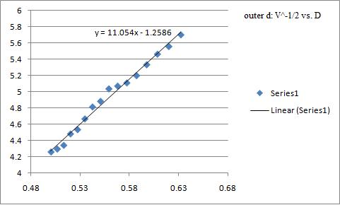
outer d: V^-1/2 vs. D


- To correct for the thickness of the glass tube, we adjusted D to be
- [math]\displaystyle{ D_{new} = D_{obs} - 3mm*D_{obs}/2L \,\! }[/math], since the radius of curvature is 1.5 mm.
- Since the electrons from the particle beam do not travel all of L, but only to the screen, we corrected L also.
- [math]\displaystyle{ L_{new} = L - 6.6cm*(1-cos(sin^{-1}(D_{obs}/2R)))\,\! }[/math].
- Using an excel spreadsheet, I calculated the average values for [math]\displaystyle{ d_{inner}\,\! }[/math] and [math]\displaystyle{ d_{outer}\,\! }[/math].
- [math]\displaystyle{ d_{inner} = 0.19524 +/- 0.001 nm\,\! }[/math]
- [math]\displaystyle{ d_{outer} = 0.11153 +/- 0.0006 nm\,\! }[/math]
Error
Calculating the percent error against the accepted values [math]\displaystyle{ d_{inner} = 0.213 nm\,\! }[/math] and [math]\displaystyle{ d_{outer} = 0.123 nm\,\! }[/math].
- [math]\displaystyle{ \% error=\frac{d_{inner}-d_{measured}}{d_{inner}}\,\! }[/math]
- [math]\displaystyle{ \% error_{inner} = 8.34 %\,\! }[/math]
- [math]\displaystyle{ \% error_{outer} = 9.33 %\,\! }[/math]
- My best best assumption for the reasons for our error for this lab was probably because of the inaccuracy in measuring the diameters with the calipers. The diameters grew fuzzier as we decreased the voltage.
Acknowledgements
- I would like to thank Ginny my lab partner for this lab because she made the graphs. You can go to her page by clicking on the link at the top of this page.
- Professor Koch for helping us understand the setup.
