Angela C Abarquez Week 11

Purpose

The purpose is to use MATLAB to simulate a chemostat experiment. The computations will be made using given parameter values and will be compared to a steady state outcome.

Background Notes

The following were noted from the Week 11 Assignment Document:

Q: volumetric inflow rate (vol/time)

q: dilution rate (q=Q/V)

- units: 1/time

- V=volume, constant

u: feed concentration

- units: concentration, mass or molar

rate of change of nutrient = inflow rate - outflow rate - rate consumed in the tank

Steady states are found by setting the right side of the DE system to 0

Methods

The MATLAB files chemostat_script.m and chemostat_dynamics.m were used to simulate a chemostat and compare the computations to a steady state outcome. The codes are in the zip file here.
The following parameter values were used: q = 0.10 (1/hr); u = 5 (g/L); E=1.5; r=0.8 (1/hr); K = 8 (g)
The formulae in the document (linked in "Data and Files" section), were used and a 2 liter chemostat was assumed.
The system dynamics using the MATLAB files and parameters in step 2 were simulated.
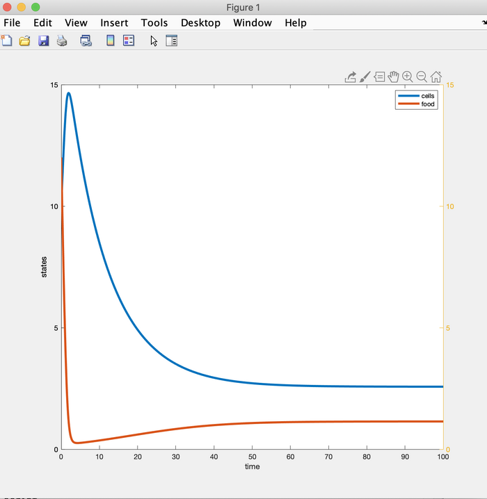
The "yyaxis right" and "ylim ([0 150])" functions were input to create the bonus graph with the y-axis labeled on both sides.

Results

What are the steady states of cell biomass and nutrient mass?

Cell biomass: 2.5748g

Nutrient mass: 1.1412g

Assuming a 2 liter chemostat, what are the steady state concentrations of cells and nutrient?

Cells: 2.5748g/2L = 1.2875g/L

Nutrient: 1.1412g/2L = 0.5706g/L

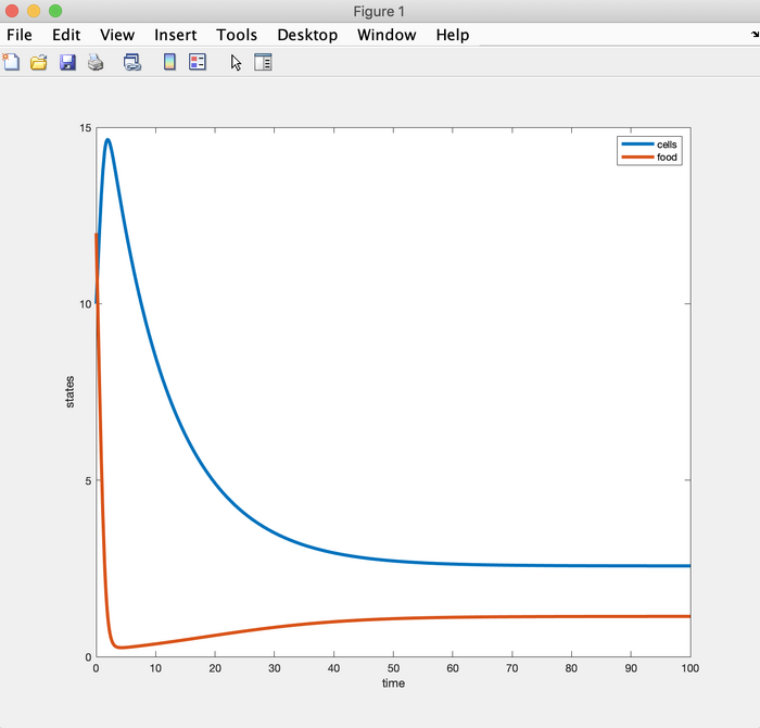
Figure 1. MATLAB plot generated from simulated chemostat experiment.

Do the graphs show the system going to steady state?

The graph shows the system going to steady state between 50-60 hours.

Do the steady states match your (1) calculations?

Yes, the steady states are close to the (1) calculations if you account for slight rounding error.

Figure 2. Bonus graph with y-axis labeled on both sides.

Data and Files

Week 11 Assignment Document

File:Abarquez Week 11 chemostat script.m.zip

Conclusion

A chemostat was simulated using MATLAB and specific parameters were used to generate a plot. Through the use of differential equations the biomass in the system, including cells and nutrients, was analyzed. By setting the differential equations equal to zero, the resulting graph showed that steady state was reached at around 50 hours, which is expected from a chemostat experiment. The steady states of the cell biomass was found to be 2.5748g, while the nutrient mass had a steady state of 1.1412g. The graph also proves that nutrients are converted to biomass before reaching steady state. Therefore MATLAB is effective at simulating chemostat experiments.

Acknowledgments

My partner Ali and I communicated via text on 4/10 to discuss the assignment.

Except for what is noted above, this individual journal entry was completed by me and not copied from another source.

Angela C Abarquez (talk) 18:44, 10 April 2019 (PDT)

References

Dahlquist, K. & Fitpatrick, B. (2019). "BIOL388/S19: Week 11" Biomathematical Modeling, Loyola Marymount University. Accessed from the "BIOL388.S19:Week 11" assignment page, linked here